
With the Metric Builder for Excel, you can create Custom Metrics to sync your Excel data with Databox.
Navigate to Metrics > Custom Metrics to access the Metric Builder for Excel. Click the green + New Custom Metric button and select your connected Excel workbook from the Data Source drop-down list.
You can create Custom Metrics using the Metric Builder for Excel via manual setup or a more advanced wizard.
- Manual setup gives you the ability to select cells and create your Custom Metrics manually, as you do with other Metric Builders like the Metric Builder for Google Sheets.
- As long as your workbook is formatted in an optimal way to sync with Databox, the wizard will also be available to provide more guidance and make it even easier to build Custom Metrics using data from your Excel workbook. The wizard option will only be available if your workbook is formatted in Columns. This is the only format that the Wizard currently recognizes and supports.
You can switch between manual setup and the wizard by clicking on the Switch to Manual Setup or Switch to Wizard buttons in the top right of the Metric Builder.
The first page in the Excel Wizard is intended to ensure we're recognizing the setup of your Excel workbook correctly by verifying the Date, Metric, and Dimension columns. Values should be numerical, while Dimensions are typically strings. Once complete, click Continue.
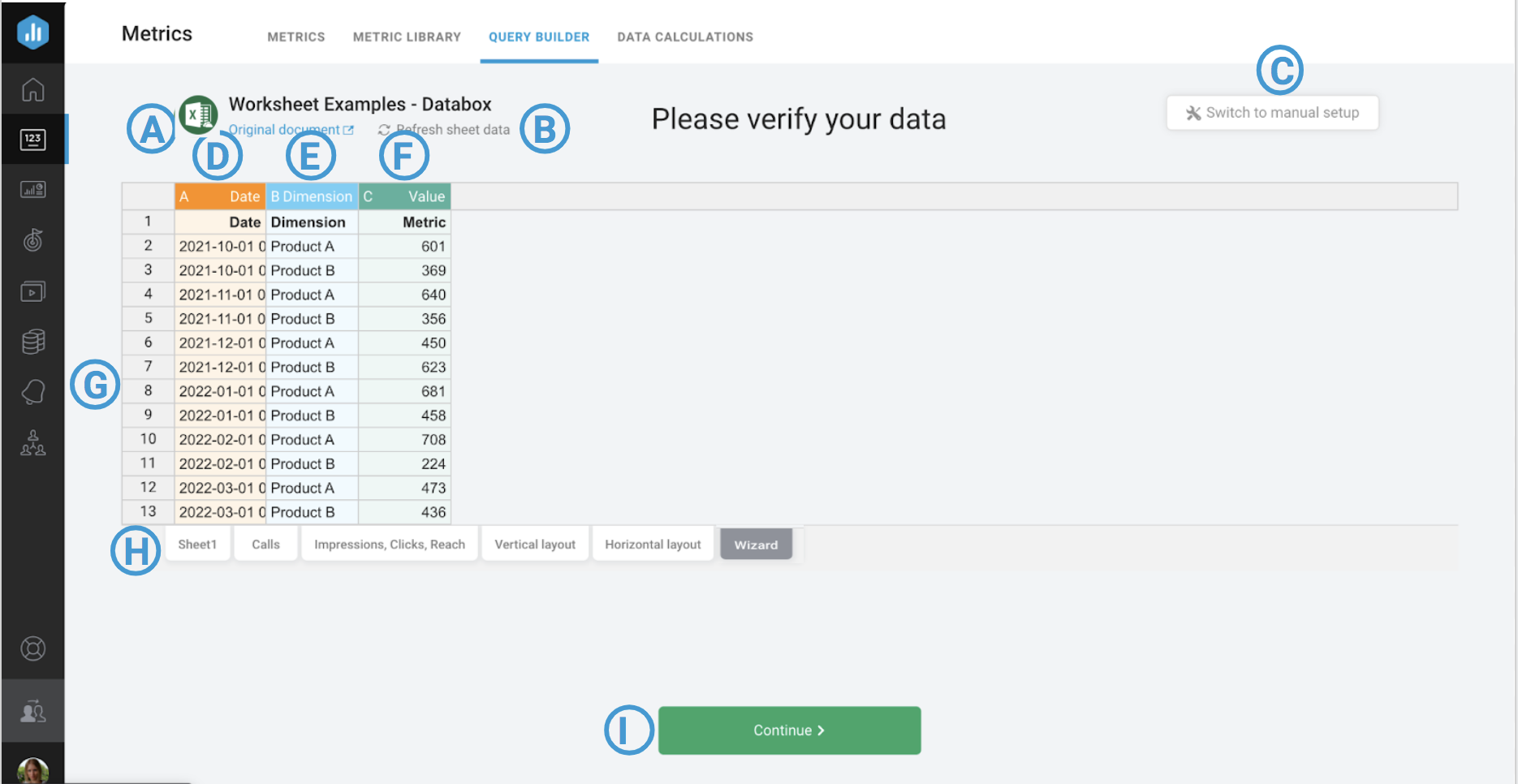
- A) Original document: The Original document link allows you to quickly access your Excel workbook to update data or make any edits you see fit.
- B) Refresh sheets data: Click Refresh sheets data if you want to see an up-to-date preview of your Excel document. This is especially beneficial if you've made changes in your Sheet.
- C) Switch to manual setup: Click Switch to manual setup if you'd like to abandon the Wizard and would prefer to select cells and set up the Custom Metric from your Excel workbook manually.
- D) Column A: Column A typically represents Dates data. Verify that this column stores the dates that your data should be pushed to. The Date needs to include information on the day, month and year that the Metric value should be pushed to. Dates in your Excel workbook should be formatted as mm/dd/yyyy, dd/mm/yyyy, mm.dd.yyyy, or dd.mm.yyyy. Learn how to format Dates in your Excel workbook to sync data with Databox here.
- C) Column B: Column B typically represents a list of Dimensions, which are strings that help categorize your metric values. For example, a Dimension may be "Source" or "Sales Rep," which would allow you to split up your metric value by Source or Rep. Dimensions are optional. Verify that this column stores the Dimensions that correspond with your metrics.
- F) Column C: Column C typically represents Metric values, which are numerical values. Verify that this column stores the Metrics in your Sheet.
- G) Excel Preview: The preview displays a live view of your Excel workbook. The first 500 rows of your Excel Worksheet will be visible in the preview, but data is synced from all rows in the Sheet.
- H) Excel Worksheets: At the bottom of the Preview, you can see the Worksheets that make up your Excel Worksheet. You can navigate between Worksheets to ensure we're recognizing and syncing the right data with Databox.
- I) Continue: Click Continueonce you've verified the setup of your Sheet to move to the next page in the Wizard.
Now that the Sheet is verified, you'll start building out the Custom Metric. To do this, you'll first select the Metric column that you'd like to use in the Custom Metric. This column should store numerical values.
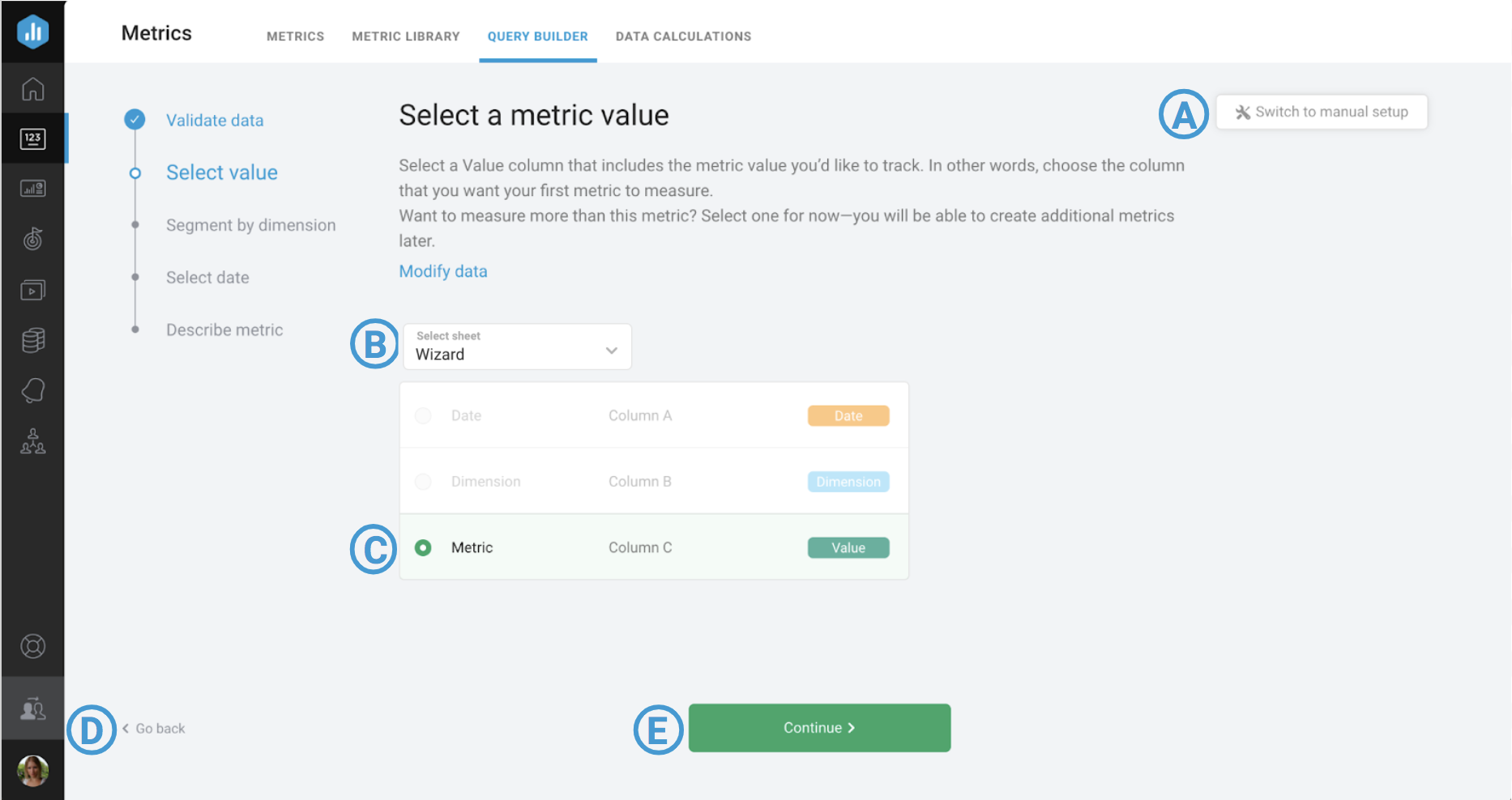
- A) Switch to manual setup: Click Switch to manual setup if you'd like to abandon the Wizard and would prefer to select cells and set up the Custom Metric from your Excel workbook manually.
- B) Select sheet: Select the Worksheet we should be syncing data from.
- C) Select Metric: Select the Metric column you'd like to use in the Custom Metric.
- D) Go Back: if you need to go back to the previous step, click Go back.
- E) Continue: Click Continue once you've verified the metric you'd like to include in your Custom Metric to move to the next page in the Wizard.
Next, we have the option of selecting a Dimension for our Custom Metric. Dimensions allow you to re-categorize the returned Metric values based on a similar attribute. Examples of Dimensions are "Country," "Source" and "Campaign." Including a Dimension is optional when building Custom Metrics. If you don't select a Dimension, just 1 value is returned for the Custom Metric. If you do select a Dimension, the metric value is split up based on the Dimension categories.
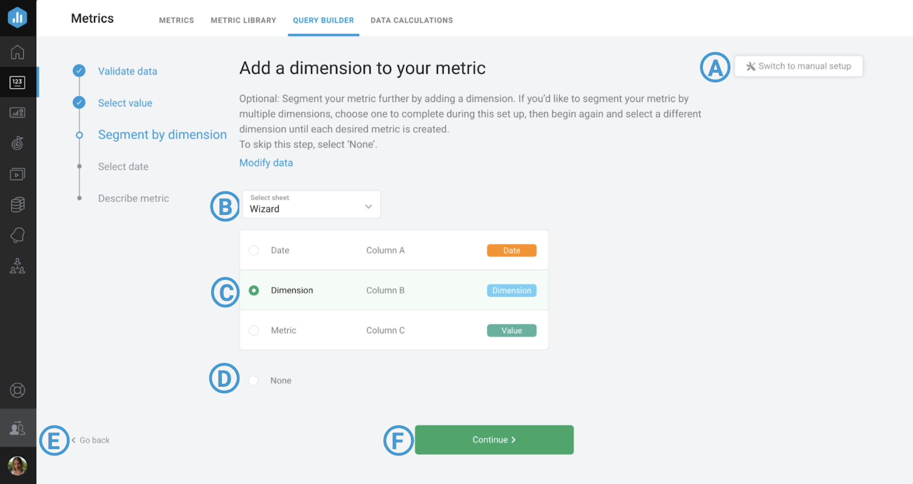
- A) Switch to manual setup: Click Switch to manual setup if you'd like to abandon the Wizard and would prefer to select cells and set up the Custom Metric from your Excel workbook manually.
- B) Select sheet: Select the Worksheet we should be syncing data from.
- C) Select Dimension: Select the Dimension column you'd like to use in the Custom Metric.
- D) None: if you don't want to include a Dimension in your Custom Metric, select None.
- E) Go Back: if you need to go back to the previous step, select Go back.
- F) Continue: Click Continue once you've verified the metric you'd like to include in your Custom Metric to move to the next page in the Wizard.
In order to display your data the way you like, you will need to include entries in your Excel workbook that specify which date(s) you want to push your data to. This enables Date Ranges to display the appropriate data in Databox.
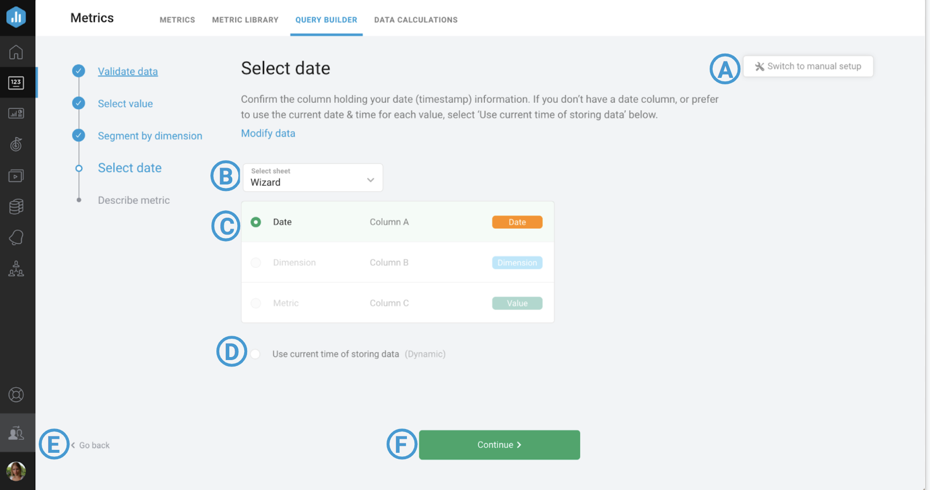
A) Switch to manual setup: Click Switch to manual setup if you'd like to abandon the Wizard and would prefer to select cells and set up the Custom Metric from your Excel workbook manually.
B) Select sheet: Select the Worksheet we should be syncing data from.
C) Select Date: Select the Date column you'd like to use in the Custom Metric.
D) Use current time of storing data: Select this option if you want your data stored based on the time it's synced with Databox.
E) Go Back: if you need to go back to the previous step, select Go back.
F) Continue: Click Continue once you've verified the metric you'd like to include in your Custom Metric to move to the next page in the Wizard.
Lastly, we need to describe and finalize the Custom Metric.
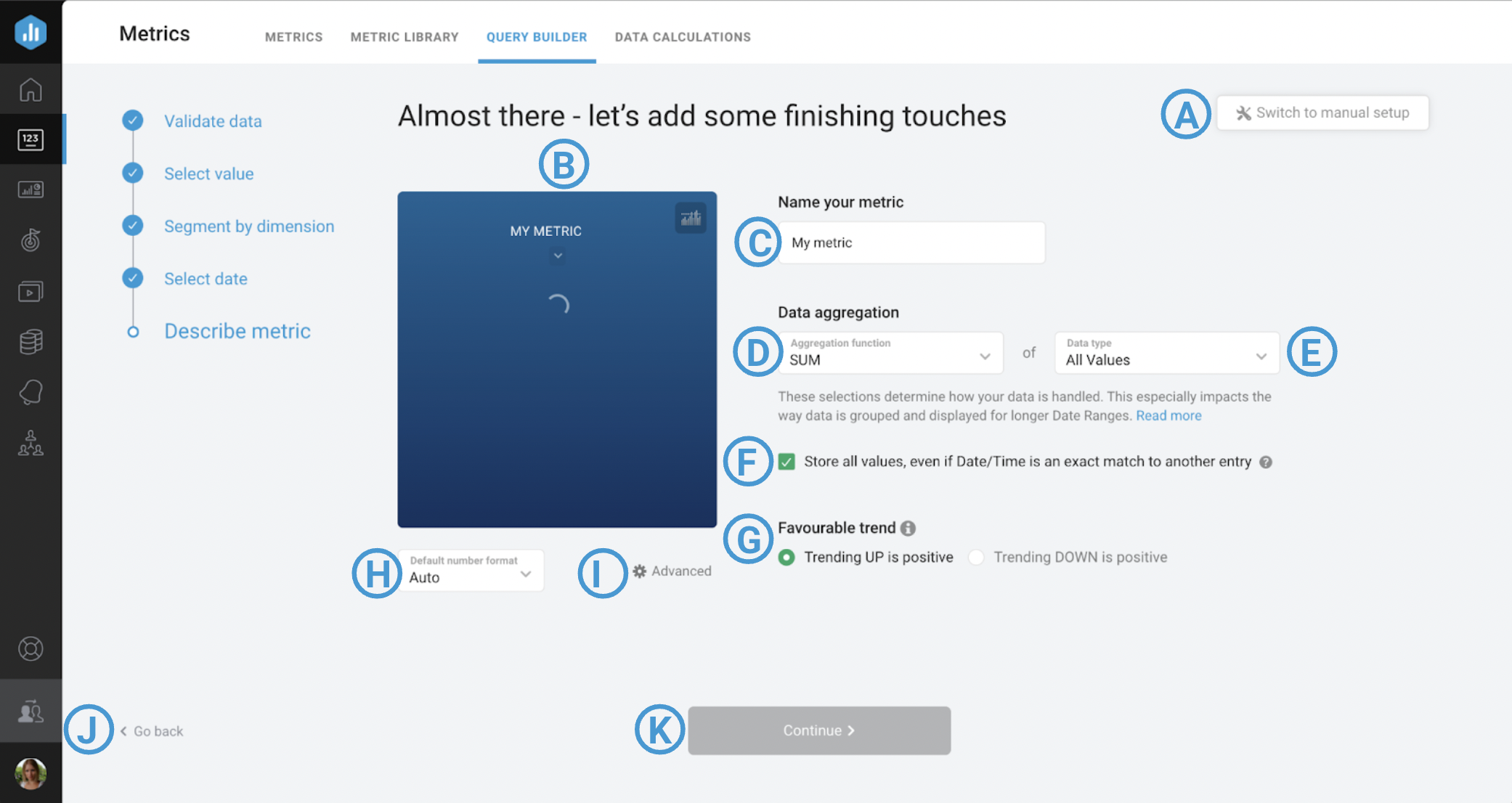
- A) Switch to manual setup: Click Switch to manual setup if you'd like to abandon the Wizard and would prefer to select cells and set up the Custom Metric from your Excel workbook manually.
- B) Data Preview: As you build your Custom Metric, a Data Preview will update to reflect your selection. You can view the Data Preview for different visualizations by clicking on the icons at the top of the Data Preview. When you save the Custom Metric, the selected visualization will be stored, and a pre-built Datablock will be generated. This Datablock will be available in the Datablock Library when the appropriate Excel Data Source is selected.
- C) Name your Custom Metric: Enter a name for your Custom Metric. This Custom Metric name will be available in the Designer after saving.
- D) Aggregation Function: Selecting the appropriate Aggregation function ensures that values for your Custom Metrics will be aggregated correctly in Databox. The Aggregation function is closely connected with the selected Data Type. Learn more here.
- E) Data Type: Selecting the appropriate Data Type ensures that your Custom Metrics will be synced correctly in Databox. The Data Type is largely dependent on the way you plan to update your Excel workbook with new data. Learn more about Data Types here.
- F) Store all Values: Select this option if you'd like all data synced with Databox, even if the date/time of the entires are identical.
- G) Favourable Trend: There are some cases where an increase in the Metric value does not signify an improvement in performance and vice versa. In those cases, an increase in the Metric value should be displayed in red while a decrease in the Metric value should be displayed in green. Select the Favourable Trend based on what defines success for your Custom Metric. Learn more here.
- H) Metric Format: Choose the Format for your Custom Metric. Learn more here.
- I) Advanced: In the Advanced window, you access additional settings to customize your Custom Metric. This includes adding a Description, changing the Data Aggregation, or updating Visual Preferences. Learn more about advanced settings for the Custom Metric here.
- J) Go Back: if you need to go back to the previous step, select Go back.
- K) Continue: Click Continue once you've verified the metric to save the Custom Metric.
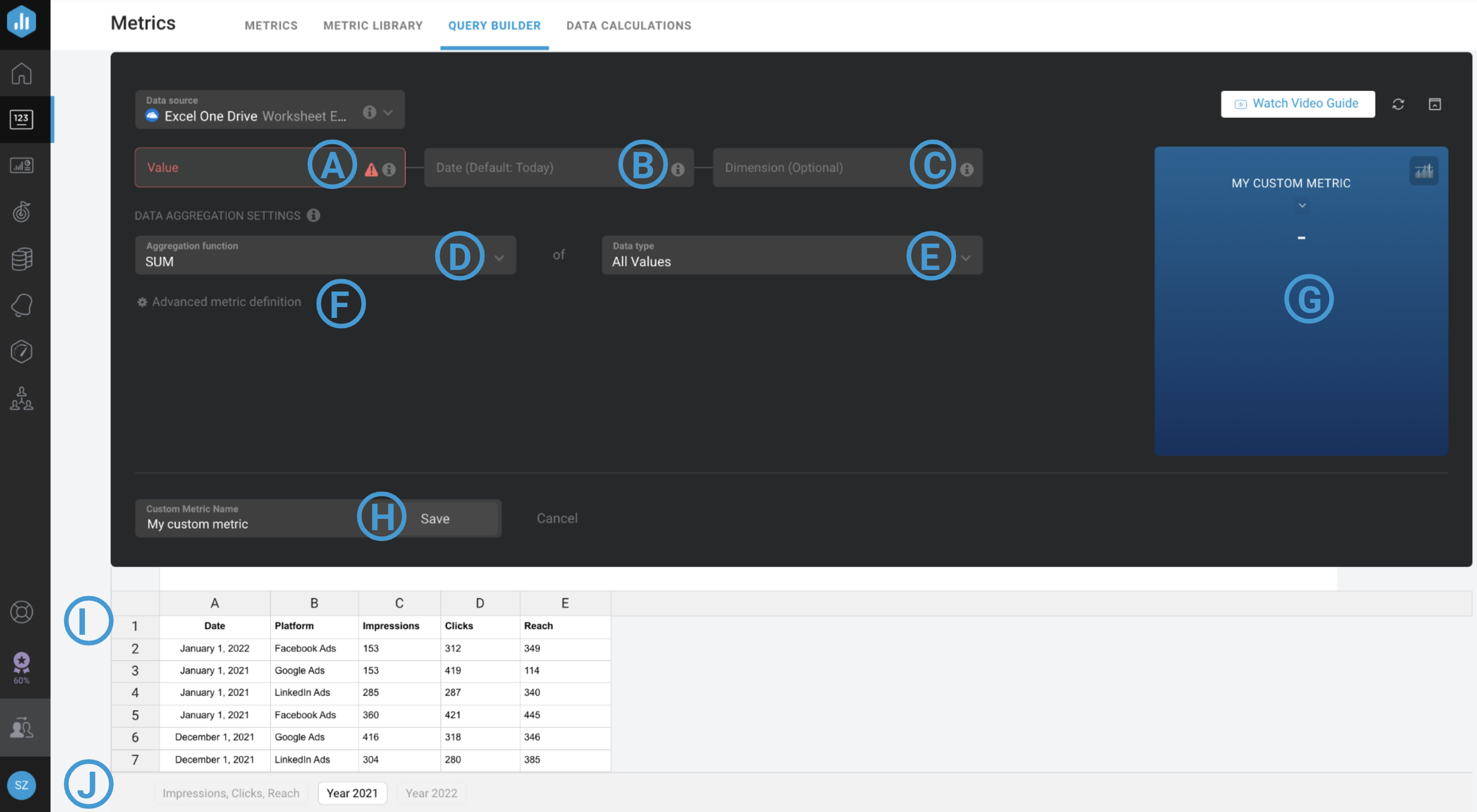
**A) Value:**Select a cell or a range of cells from your Excel worksheet that stores the Metric Value(s). These cells must contain numerical values (Currency and other Unit formats are supported). Select the cell(s) and navigate to Home > Number Format > Number in your Excel worksheet to verify that the entries are entered as Numbers and not Strings.
- A cell or a range of cells can be entered using A1 notation or by highlighting the selection directly in the Worksheet Preview section at the bottom of the Metric Builder. Learn more about A1 notation here.
- If you select an entire row or column as the Value selection, any new entries in the selected row or column will automatically sync the new data to the Custom Metric in Databox.
B) Date: To display your data the way you like, you will need to include entries in your Excel worksheet that specify which date(s) you want to push your data to. This enables Date Ranges to display the appropriate data in Databox.
To verify that your entries are entered correctly as Dates, select the cell(s) and navigate to Home > Number Format > More Number Formats > Date in your Excel worksheet. The Date needs to include information on the day, month and year that the Metric value should be pushed to. Dates in your Excel workbook should be formatted as mm/dd/yyyy, dd/mm/yyyy, mm.dd.yyyy, or dd.mm.yyyy.
- Learn how to format Dates in your Excel workbook here.
C) Dimension (Optional): The Dimension parameter re-categorizes the Metric value based on common criteria. Examples of Dimensions are Referrer, Browser, Country, and Product Name.
- Each Metric Value can support up to one associated Dimension. To use additional Dimensions from your Excel worksheet with the selected Metric Value, you need to build another Custom Metric. This means that if you want to report on Sessions by Browser and Sessions by Country, you would need to create two separate Custom Metrics in Databox.
- If no Dimension is selected, the Custom Metric will either store one aggregated Metric Value for each Date Range or the latest Metric Value. This behavior will depend on the selected Data Type.
D) Aggregation function: Selecting the appropriate Aggregation function ensures that values for your Custom Metrics will be aggregated correctly in Databox. The Aggregation function is closely connected with the selected Data Type. Learn more here.
E) Data Type: Selecting the appropriate Data Type ensures that your Custom Metrics will be synced correctly in Databox. The Data Type is largely dependent on the way you plan to update your Excel workbook with new data.
Learn more about Data Types here.
F) Advanced metric definition: Here, you can customize Custom Metric settings. This includes adding a Description, determining if all values should be stored, even if the Date/Time is an exact match to another entry, inverting the metric value (e.g., Trending down is positive), setting the Default Number Format, adjusting the Default Comparison Function, and many more settings. Learn more about advanced settings for Custom Metrics here.
G) Data Preview: As you build your Custom Metric, the Data Preview will update to reflect your selection. You can view the Data Preview for different visualizations by clicking on the icons at the top of the Data Preview.
- When you save the Custom Metric, the selected visualization will be stored, and a pre-built Datablock will be generated. This Datablock will be available in the Datablock Library when the appropriate Excel Data Source is selected. You can still choose to visualize the Custom Metric on another visualization type when building dashboards in the Databox Designer.
H) Custom Metric Name: Enter a name for your Custom Metric. This Custom Metric name will be available in the Designer after saving.
I) Excel Preview: The Excel Preview displays a live view of your Excel worksheet. You can use this Excel Preview to simplify the selection process for the Value, Date, and Dimension fields. The first 1000 rows of your Excel worksheet will be visible in the Excel Preview, but data is synced from all rows in the Worksheet.
J) Excel Worksheets: Select the Worksheet you would like to view in the Excel Preview. To make the Metric Value selection as straightforward as possible, the selected Worksheet should host the data you are syncing with the Custom Metric.
When creating Custom Excel Metrics you can use help of a wizard or you can choose to create Custom Metric manually,
Creating Custom Metric with the wizard is selected by default, as long as your Excel file is formatted in a way that Databox recognizes. You can click Switch to manual setup button if you would prefer to set up your Custom Metric manually.

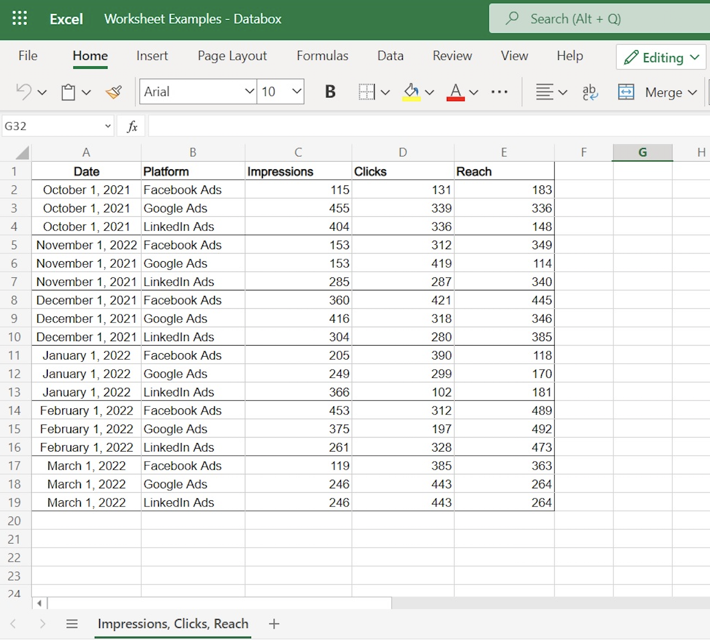
Let's say we want to create a Custom Metric to track Impressions from the Excel worksheet below.

- In the Excel Wizard, we'll verify the Date, Metric (value), and Dimension(categories) columns from our Excel worksheet. Values should be numerical, while Dimensions are typically strings. Once complete, we'll click Continue.
- Next, we'll start building the Custom Metric. First, we'll select the Value (numerical data) we want to include in our Custom Metric. In this case, we'll select Impressions (Column C) and click Continue.
- Since we don't want to include a Dimension (i.e., we just want 1 number returned to show total Impressions, we don't want it broken up by a category), we will select Noneon the Segment by Dimension page, then will click Continue.
- We need to specify the dates that this data should be pushed to. In our Sheet, this is column A. We'll select this on the Select Date page then click Continue.
- Finally, we need to add some information on the new Custom Metric we're building, including a Custom Metric name and how data should be aggregated (grouped) when it's synced with Databox. We'll name this Custom Metric Impressions, and will keep SUM of All Values selected as the Aggregation functionand **Data type.**This is because we want to add together all synced values for the metric.
- There are identical Date stamps on this Excel Sheet, and we want them all included in the Custom Metric. Therefore, we'll leave the checkbox Store all values, even if Date/Time is an exact match to another entry checked to ensure all of our data is synced correctly.
- Next, we'll select the visualization that we want to be associated with the pre-built Datablock for this Custom Metric in the Data Preview section. We are interested in analyzing the trend of this Metric, so we will select a **Line Chart.**When building Databoards, we will still be able to visualize this metric using different visualization types as we see fit.
- Click Continue to save the Custom Metric.
Let's say we want to create a Custom Metric to track Impressions by Platform from the Excel worksheet below.
- In the Excel Wizard, we'll verify the Date, Metric (value), and Dimension (categories) columns from our Excel workheet. Values should be numerical, while Dimensions are typically strings. Once complete, we'll click Continue
- Next, we'll start building the Custom Metric. First, we'll select the Value (numerical data) we want to include in our Custom Metric. In this case, we'll select Impressions (Column C) and click Continue
- We want to view Impressions split up based on the Platform they were tracked in, so we will select Platform (Column B) as the Dimension and click Continue
- We need to specify the dates that this data should be pushed to. In our Sheet, this is column A. We'll select Date (Column A) on the Select Date page then click Continue
- Finally, we need to add some information on the new Custom Metric we're building, including a Custom Metric name and how data should be aggregated (grouped) when it's synced with Databox. We'll name this Custom Metric Impressions by Platform, and will keep SUM of All Values selected as the Aggregation functionand Data type. This is because we want to add together all synced values for the metric, based on the Dimension (Platform)
- There are identical Date stamps on this Excel Sheet, and we want them all included in the Custom Metric. Therefore, we'll leave the checkbox Store all values, even if Date/Time is an exact match to another entry checked to ensure all of our data is synced correctly
- After that, we'll select the visualization that we would like associated with the pre-built Datablock for this Custom Metric from the Data Preview section. We are interested in analyzing the distribution of Impressions across the Platforms, so we will select a **Pie Chart.**When building Databoards, we will still be able to visualize this metric using different visualization types as we see fit
- Click Continue to save the Custom Metric
The Switch to wizard button is greyed out if the data in your Excel file is not structured in columns. This is a requirement in order to be able to use Metric Builder for Excel wizard. Learn how to structure data in columns in your Excel file here.
If you don't want to restructure the data in your Excel file, follow the steps outlined below to create your Custom Excel Metrics via manual setup.
Let's say we want to create a Custom Metric to track Impressions from the Excel worksheet below.


- In the Excel Worksheet Preview, we'll select column C as the Value. Since we are selecting the full column, any additional Values added to this column of the worksheet will be automatically synced with Databox.
- Next, we'll select the Datecolumn from our Excel worksheet, which is column A.
- This Metric does not need a Dimension, so we will leave the Dimension field blank.
- We want to get the sum of all values per selected Date Range. So, we'll leave SUM as the Aggregation Function .
- We want all values synced with Databox, so we'll leave All Values as the Data Type.
- There are identical Date stamps for entries included in this Excel worksheet, but we want them all included in the Custom Metric. We'll navigate to Advanced metric definition > Data Aggregations tab and select the Store all values, even if Date/Time is an exact match to another entry checkbox to ensure all of our data is synced correctly.
- Next, we'll select the visualization that we would like associated with the pre-built Datablock for this Custom Metric from the Data Preview section. We want to analyze the trend of this Metric, so we will select a **Line Chart.**We can still select other visualization types when visualizing the Custom Metric on dashboards.
- We'll enter Impressions as the Custom Metric Name.
- Pro Tip: Typically, the Custom Metric Name is the same as the column or row header from the Excel worksheet.
- Finally, we'll click Saveto save the Custom Metric.
Let's say we want to create a Custom Metric to track Impressions by Platform from the Excel worksheet below.

- In the Excel Worksheet Preview, we'll select column C as the Value. Since we are selecting the full column, any additional Values added to this column of the worksheet will be automatically synced with Databox
- Next, we'll select the Date column from our Excel worksheet, which is column A.
- We want to view Impressions split up by the Platform they were tracked in, so we will select column B(Platform) as the Dimension.
- We want to get the sum of all values per selected Date Range. Therefore, we'll leave the SUMas the Aggregation function.
- We want all values synced with Databox, so we'll leave All Values as the Data Type.
- There are identical date stamps on this Excel worksheet. Therefore, we'll navigate to the Advanced metric definition > Data Aggregations tab and select Store all values, even if Date/Time is an exact match to another entry checkbox, to ensure all of our data is synced correctly
- There are identical Date stamps for entries included in this Excel worksheet, but we want them all included in the Custom Metric. We'll navigate to Advanced metric definition > Data Aggregations tab and select the Store all values, even if Date/Time is an exact match to another entry checkbox to ensure all of our data is synced correctly.
- Next, we'll select the visualization that we would like associated with the pre-built Datablock for this Custom Metric from the Data Preview section. We are interested in analyzing the distribution of Impressions across the Platforms, so we will select a **Pie Chart.**We can still select other visualization types when visualizing the Custom Metric on dashboards.
- We'll enter Impressions by Campaign as the Custom Metric Name
- Pro Tip: Typically, the Custom Metric Name is the same as the column or row header from the Excel worksheet, with "by" in between the Value and Dimension selections.
- Click Save to save the Custom Metric
- Open the selected Databoard in the Databox Designer, or create a new Databoard.
- Click on the Metric****Library icon on the lefthand side of the Designer.
- Select the Excel workbook for which you want to view Datablocks from the Data Source drop-down list. The Custom Metrics that have been created for the Excel worksheet(s) will populate the Metric Library.
- Find the Datablock you want to add to your Databoard, using the Searchbar if necessary.
- Drag and drop the selected Datablock onto your Databoard. The Datablock will automatically populate with data from the Excel workheet that was selected in the Metric Library.
- Open the selected Databoard in the Databox Designer, or create a new Databoard
- Click on the Visualization Types icon on the lefthand side of the Designer
- Find the Visualization you want to add to your Databoard
- Drag and drop the selected Visualization onto your Databoard. Use the righthand Datablock Editorpanel to populate the Datablock
- Each Excel Custom Metric supports only one data Aggregation function. To view the same Excel Custom Metric with different Aggregation functions selected (i.e., "SUM" on one vs. "AVG" on another), duplicate Custom Metrics and create the views you desire by following these steps.