
Databox offers a robust feature for detecting outliers in the data, developed by its Data Science team using the advanced Facebook Prophet model. This feature analyzes historical data and relevant factors to accurately identify anomalies.
Anomalies are data points that deviate from expected variability. While fluctuations in business metrics are normal, it's important to distinguish between routine variations and true anomalies. Databox's statistical model estimates expected variability from historical data, helping to filter out random noise and focus on significant deviations that require attention.
The model detects anomalies through a three-stage process:
- Data analysis: The model is trained on historical data, breaking it down into components such as trend, seasonality, and events.
- Estimating expected variation: Using this analysis, the model calculates the expected range of variation for a given metric.
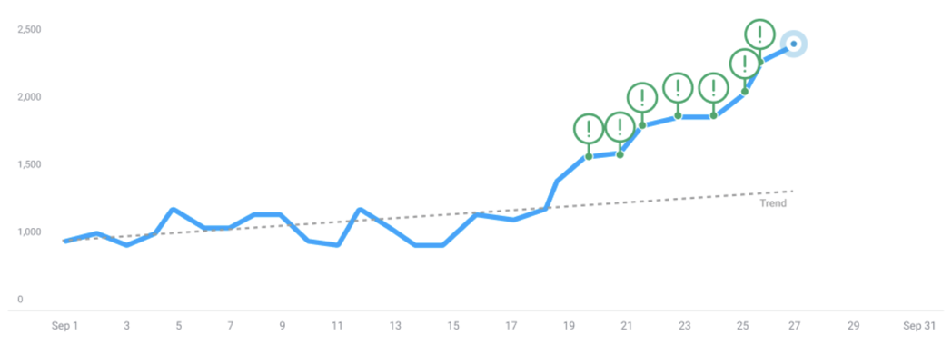
- Identifying anomalies: Any metric values falling outside the expected range of variation are flagged as anomalies.
The first step in anomaly detection is training the model on the available data. This involves developing a model that identifies patterns in the data and estimates the expected variations around those patterns.
Databox's anomaly detection model allows flexibility in training, either using only the observed date range or extending it by including additional historical data points before the observed period.
Extending the training period often improves the accuracy and reliability of anomaly detection by providing a more complete view of trends, seasonal patterns, and event impacts. This helps define more precise variation ranges, enhancing the model's ability to distinguish between normal fluctuations and actual anomalies.
However, if there has been a significant shift in the data, making older data less relevant, it is recommended to exclude that data from the training period.
Trends are sequences of consecutive data points that show consistent behavior, such as increasing, stable, or decreasing patterns. While some metrics may exhibit a stable average value, leading to a consistent trend, others may show dynamic changes, resulting in varying trends or patterns. Recognizing and accounting for these variations is crucial for accurately understanding the data.
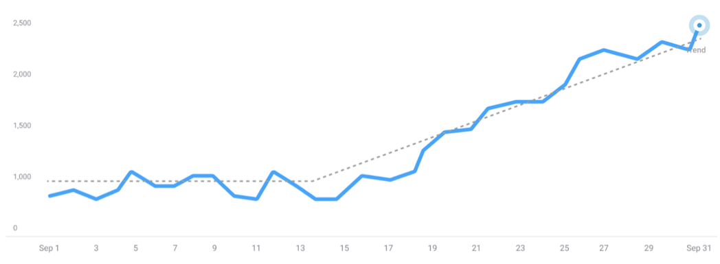
For example, if a metric was constant until a certain point, after which it starts to increase linearly due to a successful intervention, the model must adapt to these changing trends. Without this adjustment, the model might mistakenly classify some of the new data points as anomalies.
Trends can evolve over time, and the model adapts to new information as it becomes available. As new data points are recorded, the model recognizes shifts in trends, such as linear growth becoming the 'new normal.' It updates its calculations and adjusts its trend estimates to reflect these changes. Consequently, data points that were previously classified as anomalies may no longer be considered anomalous, as they now fall within the updated 'new normal' established by the additional data:
Additional data points prompt the model to recalculate and adjust its trend estimates and expectations. For instance, with the introduction of new data points, the model may identify more changepoints and recognize multiple trends:
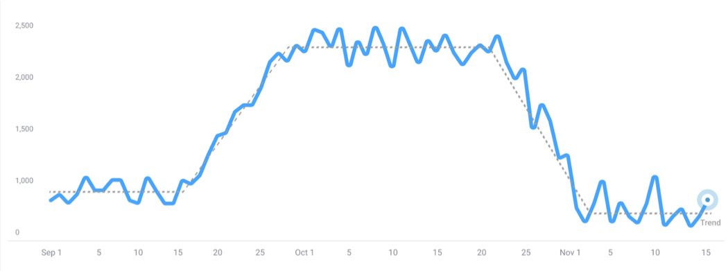
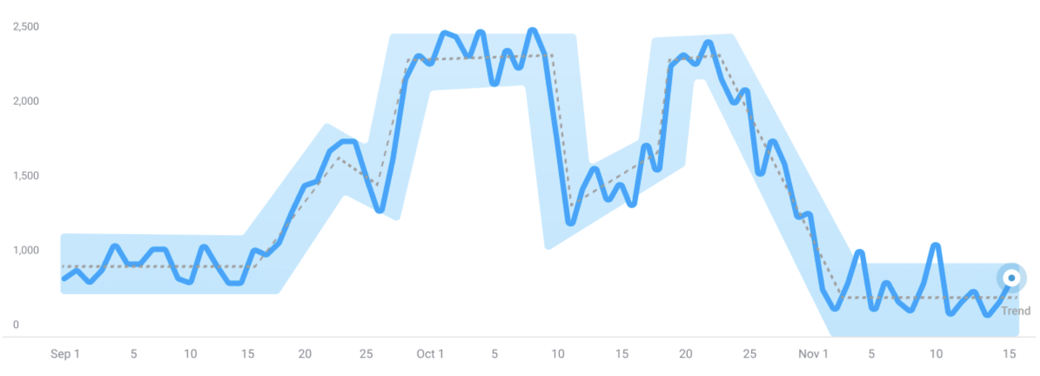
The model's adaptability settings control how many changepoints it identifies. A model with high adaptability will detect short-term changes, capturing multiple changepoints and trends within the time series. Conversely, a model with low adaptability will identify fewer changepoints, resulting in a more stable trend that doesn't account for short-term variations.
Example of a low adaptability model:
Example of medium adaptability model:
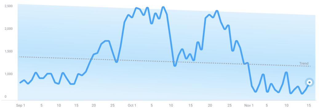
Example of a high adaptability model:
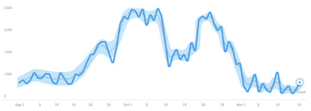
A highly adaptable model generally leads to a narrower expected range of variation. This occurs because such a model adjusts closely to the data, capturing the trend with minimal variability. In contrast, a less adaptable model leads to greater variability around the trend, as it is less responsive to data changes, resulting in a broader range of variation.
The model calculates expected variation by generating in-sample forecasts for the historical period based on learned patterns. It estimates what the values should have been and computes uncertainty intervals for each historical data point, factoring in uncertainties related to trend and seasonal variations.
Using these estimations, prediction ranges (e.g., 80% or 95% confidence ranges) are established to represent the expected span within which actual historical values should fall. The model then compares actual historical values to these predicted ranges. Any value that falls outside these ranges is flagged as an anomaly, indicating a significant deviation from the expected range based on learned patterns and estimated uncertainties.
The sensitivity setting controls the width of the expected variation range in the model. By default, the model is calibrated so that around 1% of data points fall outside this range under normal conditions, meaning it may incorrectly flag 1% of regular data as anomalies while still capturing true anomalies with high confidence. The sensitivity parameter can be adjusted to widen or narrow the expected variation range, thereby classifying more or fewer points as anomalies.
Anomalies are data points that fall outside the expected variability range. Under normal conditions, all variation is expected to remain within this range. Any point outside this range signals special circumstances that may require attention.
To aid in the detection process, the model assigns an anomaly score to each identified anomaly. This score quantifies the degree of deviation from the expected variability range, based on the distance between the observed value and the nearest boundary of the expected variability range. A higher anomaly score reflects a greater deviation, indicating a more significant anomaly. Scores are normalized on a 0-100 scale.