
Localization is the process of customizing content, formatting, and other elements to align with your language or regional preferences. This ensures that the data is accurately interpreted and displayed. By localizing your files, you can ensure that external services like Databox can access and utilize this information correctly through various APIs.
Date and number formats differ globally. Adapting your file locally aligns these formats with your region, ensuring clear and consistent presentation of dates and numbers.
Let's consider the date December 5th, 2023:
- In the United States, this date is typically represented as 12/05/2023 (MM/DD/YYYY), indicating the month (December) first, followed by the day (5th), and then the year (2023).
- In many non-US locales like the UK or Europe, the same date would be represented as 05/12/2023 (DD/MM/YYYY), where the day (5th) comes before the month (December), followed by the year (2023).
- Navigate to File > Settings. This
- will open the spreadsheet settings pop-up window.
- In the pop-up window, find the Locale dropdown menu. Click on it to reveal a list of available locales.
- Scroll through the list and select the language or region that matches your preferences. This selection will adjust the date, time, currency, and number formats to align with that specific locale.
- After selecting your desired locale, click the Save and reload button in the bottom-right corner of the window to apply the changes. Your Google Sheet will now reflect the chosen locale settings.
The steps may differ depending on the version of Excel you are using.
If you are using Excel for the web, you can find a dedicated article on this topic in the official documentation, available here.
If you are using a desktop version, the steps might slightly vary, but the general process remains similar.
For Windows:
- Click on the upper-left corner of the worksheet (where the row numbers and column letters meet) to select the entire workbook.
- Right-click within the selected area, and choose Format Cells from the context menu. Alternatively, go to the "Home tab" on the ribbon, click the dialog box launcher icon (small square with an arrow) in the "Number" group to open the "Format Cells" dialog box.
- In the "Format Cells" dialog box, navigate to the Number or Date category based on what you want to modify.
- Select the desired format from the list or customize it using the available options.
- Once you've selected the desired format, click OK to apply the format changes to the entire selected range or workbook.
For Mac:
- Click on the upper-left corner of the worksheet (where the row numbers and column letters meet) to select the entire workbook.
- Go to the Home tab on the ribbon and navigate to Format > Cells.
- In the "Format Cells" dialog box, select the Number or Date category based on what you want to modify.
- Select the desired format from the list or customize it using the available options.
- Once you've selected the desired format, click OK to apply the format changes to the entire selected range or workbook.
Orientation refers to the arrangement of information, determining how attributes and entries are organized within the document. It involves structuring data either vertically, where attributes are represented by columns and entries are arranged in rows, or horizontally, where entries are columns and attributes align vertically. This orientation establishes the layout of the spreadsheet, influencing how data is entered, sorted, filtered, and analyzed within categories or across multiple attributes.
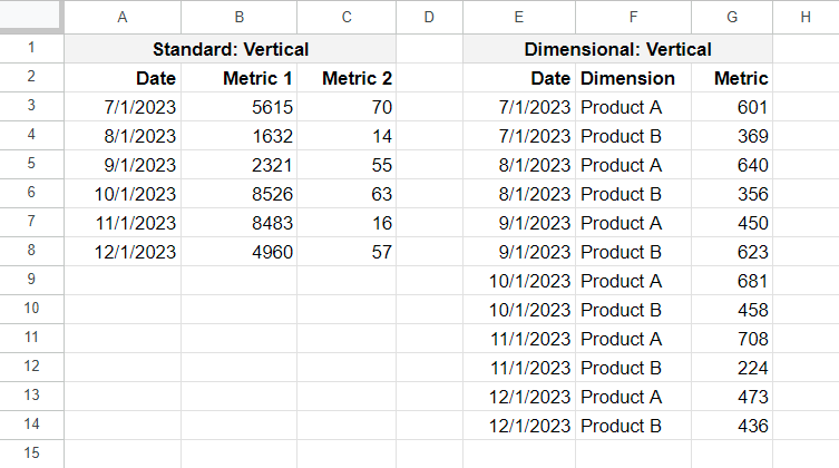
In a spreadsheet, the vertical orientation means putting information into columns. Each column contains data related to a specific category or attribute, and individual entries or records are placed in rows within these columns.
When data is organized vertically:
- Columns represent values, categories or attributes: Each column header typically denotes a specific category of information. For example, in a spreadsheet tracking sales data, columns might include "Date," "Product Name," "Quantity Sold," "Unit Price," "Total Sales," etc.
- Each row contains individual entries: Rows correspond to individual records or entries within the dataset. For instance, if the spreadsheet tracks sales, each row would represent a separate sale, with information about the date, product, quantity, price, and total sales for that transaction.
Example:
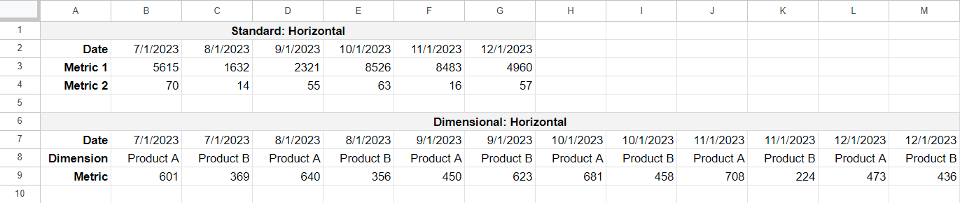
Conversely, the horizontal orientation involves arranging data by columns where individual entries or records are added as columns, and specific information within those entries is organized vertically. Each column represents a unique entry or category, while different rows contain various attributes or details related to that entry.
When data is arranged horizontally:
- Each column contain individual entries: Each column contains specific information about an entry or record. For instance, if the spreadsheet tracks sales, each column would represent a separate sale, with information about the date, product, quantity, price, and total sales for that transaction.
- Rows represent values, categories or attributes: Rows in the horizontal layout represent different types of information or attributes. For example, in a spreadsheet tracking sales data, rows might include "Date," "Product Name," "Quantity Sold," "Unit Price," "Total Sales," etc.
Example:
Formatting refers to the customization and appearance adjustments applied to the data, cells, or entire sheets to enhance readability, presentation, and analysis. It encompasses a wide range of modifications such as changing date and number formats, font styles, font sizes, colors, alignment, cell borders, and conditional formatting rules.
To effectively generate reports using Databox, it's crucial to carefully consider and ensure the compatibility of the date and number formats utilized within the document.
In Databox, every value must be linked to a specific date and time. If the date doesn't include time information, it defaults to midnight for that particular day.
We strongly recommend you ensure all dates within your data are recognized by the document, either automatically following the locale settings or manually by applying custom date formats that supersede the locale's settings. This practice significantly minimizes the chance of facing issues down the line.
There are two ways you can check whether a date is being recognized by the document:
- Text alignment on input: By default, dates are typically aligned to the right upon input if they are recognized by the document. If you observe a different alignment, it's probable that the date is being interpreted as plain text rather than a recognized date format.
- Function validation: A function can be used to verify whether a date string is being accurately interpreted by the document.
- On a Google Sheet, ISDATE() will return TRUE if the cell contains a valid date.
- On an Excel file, ISNUMBER() will return TRUE if the cell contains a valid date.
Should a date string remain unrecognized by the document, Databox will try to validate it against widely used standards such as ISO 8601 and RFC 2822.
For simplicity, we recommend adopting popular formats such as:
- YYYY-MM-DD
- MM/DD/YYYY
- DD/MM/YYYY
- December 4, 2023
- 4 December, 2023
To ensure the document recognizes your values as valid numbers and conforms to the locale settings, you should format numerical values using supported presets such as Number, Percent, Currency, Accounting, etc., or by employing a customized format.
To check if a value is recognized as a number by the document, you can make use of the ISNUMBER() function. This function will return TRUE if the cell contains a valid number.
If not explicitly formatted, numerical values will be considered valid only if they consist solely of numbers and the decimal dot (.). Additionally, all numerical values must satisfy the following criteria:
- The whole part of the number does not exceed 16 digits.
- The decimal precision does not exceed 6 digits.
Databox automatically identifies numbers formatted in specific currencies like the United States Dollar ($), Euro (€), British Pound Sterling (£), Japanese Yen (¥), and Russian Ruble (₽). For other currency formats, their symbols will be displayed in the Unit selector in-app instead of the usual three-letter codes like USD or EUR.
If you are using other measurement units (weight, duration, speed, etc.) we recommend removing this information from the cells holding the value and instead leverage the in-app formatting functionality.
Our system is designed to handle and store a specific set of information for each Metric. This includes a date, a numerical value, and the option to include a dimension and a unit. In order for Metrics to be displayed properly in our visualizations, they must have a numerical value.
If you are working with text data or data that doesn't have a numerical representation, there is one option available. You can count the number of rows or columns that meet a specific criteria and create a numerical value based on that count. This numerical value can then be displayed in our visualizations.
At this time, it is not possible to directly visualize raw tabular data or associate more than one non-numerical value (dimension) with a single value. However, we are constantly working to improve our capabilities, so please check back for any updates in the future.
Currently, Databox does not support data that is formatted or combined in pivot tables.
When analyzing data from a spreadsheet, our system expects each metric data point to have the same number of cells for its date, value and dimension components. For example, if you choose a range of 7 cells for the date, you should also select 7 cells for the value and dimension, if applicable.
Pivot tables organize data in a way that allows one date to be connected with multiple values and/ or dimensions, which disrupts the required 1:1 relationship for each data point's components.
To analyze data structured as pivot tables, we suggest converting these tables by unpivoting them. This process involves arranging the data either vertically or horizontally, as detailed in the section above.
As mentioned earlier, when displaying Metrics in our visualizations, it is necessary to have a numerical value. However, if your data does not include any numerical component, there is still an option available to work with it. You can count the number of rows or instances where a specific value is found within a Date Range. To do this, simply add a new column to the sheet and fill the cells with the number 1 if they are to be counted, or 0 if not.
Let's consider an example. Suppose you have a sheet that collects responses from one or more forms. By adding a new column with a 1 or 0, you can create a Metric in Databox to count the total number of submissions and the number of submissions by form. This allows you to visualize and analyze the data, even if it does not have a numerical representation.
To ensure compatibility with Databox, data formatted as Duration ([hh]:[mm]:[ss]) needs to be converted into seconds as Databox recognizes time durations only in seconds. Once converted, our system will then aggregate it back into minutes and hours depending on the chosen visualization format.
The conversion can be done in two ways:
- Using a formula:
Multiply the duration value by 86400.
Format the result as a Number or use a custom number format.
- Using a custom format:
- In Google Sheets, navigate to Format > Custom date and time > Elapsed seconds.
- In Excel**,** open Format Cells > Number > Custom and enter [s].
If you're dealing with various currencies in your data or you simply want to change values from one currency to another, both Google Sheets and Excel offer tools that can help you easily perform these currency conversion calculations.
In Google Sheets: To retrieve currency exchange rates and perform conversions, you can utilize the GOOGLEFINANCE() function. Simply input the function with the syntax GOOGLEFINANCE("currency:<source_currency><target_currency>") to get the desired exchange rate for your calculation.
The calculation cell might display a long decimal. You can format the cell to display the result in the desired currency format.In Excel: For detailed instructions and step-by-step guidance, you can refer to the Microsoft documentation available here.
Databox doesn't support automatic display or conditional calculations for values such as remaining business days in the calendar year. To address this, you can use the NETWORKDAYS() function as explained below.
Add a list of holidays or dates you would like to exclude from calculation to the sheet.
Add one more dates you would like to run this calculation for.
In the column next to this list of dates, add an ARRAYFORMULA() function to the top cell to calculate across all rows at once.
To calculate the remaining business days until December 31, 2024, based on a list of holidays in column C and dates in column A, you can use the following formula:
=ARRAYFORMULA(NETWORKDAYS(A1:A,DATEVALUE("2024-12-31"),D1:D)
Our system currently allows you to report on only one dimension at a time. However, if you want to analyze your data in more detail by drilling down into multiple dimensions, you can achieve this by combining or grouping all the dimensions into one value. To do this, you can use the CONCATENATE() function.
For instance, let's say you have an eCommerce website and you want to analyze your numbers by country and then by product within each country. In order to accomplish this, you would need to combine the country and product dimensions into one combined value.
In some cases, you may want to apply filters to your reports to include or exclude specific data. This allows you to focus on the information that is most relevant to your analysis. However, Databox does not currently support filtering data after it is imported. As a result, any filtering needs to be done directly in the spreadsheet before creating the Metric in Databox.
Powerful tools for extracting only a subset of data from a sheet, table or range of cells are the QUERY() function in Google Sheets and FILTER() function in Excel.
Let's say you have sales numbers grouped by payment method and you want to exclude Gift Card sales from your Metric
 In Google Sheets, enter the following in an empty cell:
=QUERY(A1:C10,"SELECT * WHERE B != 'Gift Card'")This formula uses QUERY() to select all columns (*) where the Payment Method column (B) does not equal 'Gift Card'. Here's what each parameter signifies:
- A1:C10: Specifies the range of data to be queried (from cell A:1 to C:10).
- "SELECT * WHERE B != 'Gift Card'": Defines the query to select all columns (*) where the Payment Method column (B) does not match 'Gift Card'.
After entering this formula, the result will display the filtered data in columns A, B, and C, showing only the rows where the Product column does not match 'Gift Card'.
You can also accomplish the same result in Excel by using the FILTER() function. Here is the equivalent formula for the example above:
=FILTER(A1:C10, B1:B10<>"Gift Card")You can modify the function to suit different conditions or requirements based on your dataset.


